An overview of the GWR code

This page provides a quick introduction to the new GWR driver of ABINIT We discuss the technical details related to the implementation, the associated input variables. as well as the pros and cons with respect to the conventional GW implementation formulated in Fourier-space and real-frequency domain that in what follows will be referred to as conventional or legacy GW code.

WARNING : THIS TUTORIAL IS WORK IN PROGRESS ! IT IS NOT YET COMPLETE …

Why a new GW code?

The conventional GW code has quartic scaling with the number of atoms whereas GWR scales cubically. The legacy GW code obtains the self-energy matrix elements by performing a convolution in frequency domain, (by default with the plasmon-pole approximation) whereas GWR computes the self-energy matrix elements in imaginary-time followed by an analytic continuation to the real-frequency axis.

The conventional GW code presents quartic scaling with the number of $\qq$-points whereas GWR has linear scaling. The legacy GW code can parallelize the computation over the nband states using MPI but other datastructures such as the screened interaction W is not MPI-distributed. As a consequence the maximum number of MPI processes that can used is limited by nband and the workload is not equally distributed when the number of MPI processes does not divide nband. Most importantly, the self-energy computation in the legacy version is rather memory-demanding as one has to store in memory both the wavefunctions (whose memory scales) as well as $W$ (non scalable portion). This renders self-energy calculatins rather difficult when one has to deal with large %npweps and/or computations beyond the plasmom-pole approximation in which one needs to store in memory the $W$ matrix for several frequencies.

In the GWR code, on the contrary, most of the datastructures are MPI distributed although this leads to many more MPI communications in certain parts of the algorithm. More specifically, GWR uses PBLAS to distribute the memory required to store the Green’s functions and $W$ and this allows one to tackle larger systems if enough computing nodes are availab.e is able to distribute the points along the imaginary axis, the

Select the task to be performed when optdriver == 6 i.e. GWR code. while gwr_task defines the task to be performed.

Requirements

First of all, one should mention that the GWR code requires an ABINIT build with Scalapack enabled. Moreover, a significant fraction of the computing time is spent in doing FFTs thus we highly recommend to use optimized external FFT libraries such as MKL-DFTI or FFTW3.

Discuss single and double precision version. single-precision is the default To run GWR calculations in double-precision, remember to configure with –enable-gw-dpc=”yes” or the enable_gw_dpc=”yes”.

Formalism

The zero-temperature Green’s function in imaginary-time is given by:

$$\begin{equation} G(\rr, \rr', i\tau) = \Theta(\tau) \Gove(\rr, \rr', i\tau) + \Theta(-\tau) \Gund (\rr, \rr', i\tau) \end{equation}$$

with $\Theta$ the Heaviside step-function and

$$\begin{equation} \Gove(\rr, \rr', i\tau) = -\sum_n^{\text{unocc}} \psi_n(\rr)\psi_n^*(\rr') e^{-\ee_n\tau} \qquad (\tau > 0) \end{equation}$$

$$\begin{equation} \Gund(\rr, \rr', i\tau) = \sum_n^{\text{occ}} \psi_n(\rr)\psi_n^*(\rr') e^{-\ee_n\tau} \qquad (\tau < 0) \end{equation}$$

For simplicity, we assume a spin-unpolarized semiconductor with scalar wavefunctions (i.e. [[nsppol] = 1 with nspinor = 1) and the Fermi level $\mu$ is set to zero.

The GWR code constructs the Green’s function from the KS wavefunctions and eigenvalues stored in the WFK file specified via getwfk_filepath (getwfk in multi-dataset mode). This WFK file is usually produced by performing a NSCF calculation including empty states and the GWR driver provides a specialized option to perform a direct diagonalization of the KS Hamiltonian in parallel with Scalapack. (see section below) When computing $G^0$, the number of bands included in the sum over states is controlled by nband. Clearly, it does not make any sense to ask for more bands than the ones available in the WFK file.

The imaginary axis is sampled using a minimax mesh with gwr_ntau points. The other piece of information required for the selection of the minimax mesh is the ratio between the fundamental gap and the maximum transition energy i.e. the differerence between the highest KS eigenvalue for empty states that clearly depends on nband and the energy of the lowest occupied state.

Note that only $\Gamma$-centered $\kk$-meshes are supported in GWR, e,g:

• ngkpt 4 4 4
• nshiftk 1
• shiftk 0 0 0

The cutoff energy for the polarizability is given by ecuteps while ecutsigx defines the number of g-vectors for the exchange part of the self-energy.

Note that GWR also needs the GS density produced by a previous GS SCF run. The location of the file can be specified via getden_filepath.

$$\begin{equation} \chi(\rr,\RR', t) = G(\rr,\RR', i\tau) G^*(\rr,\RR', -i\tau) \end{equation}$$

As concerns the treatment of the long-wavelenght limit, we have the following input variables:

inclvkb, gw_qlwl, gwr_max_hwtene

GWR workflow for QP energies

A typical GWR workflow with arrows denoting dependencies between the different steps is schematically represented in the figure below:

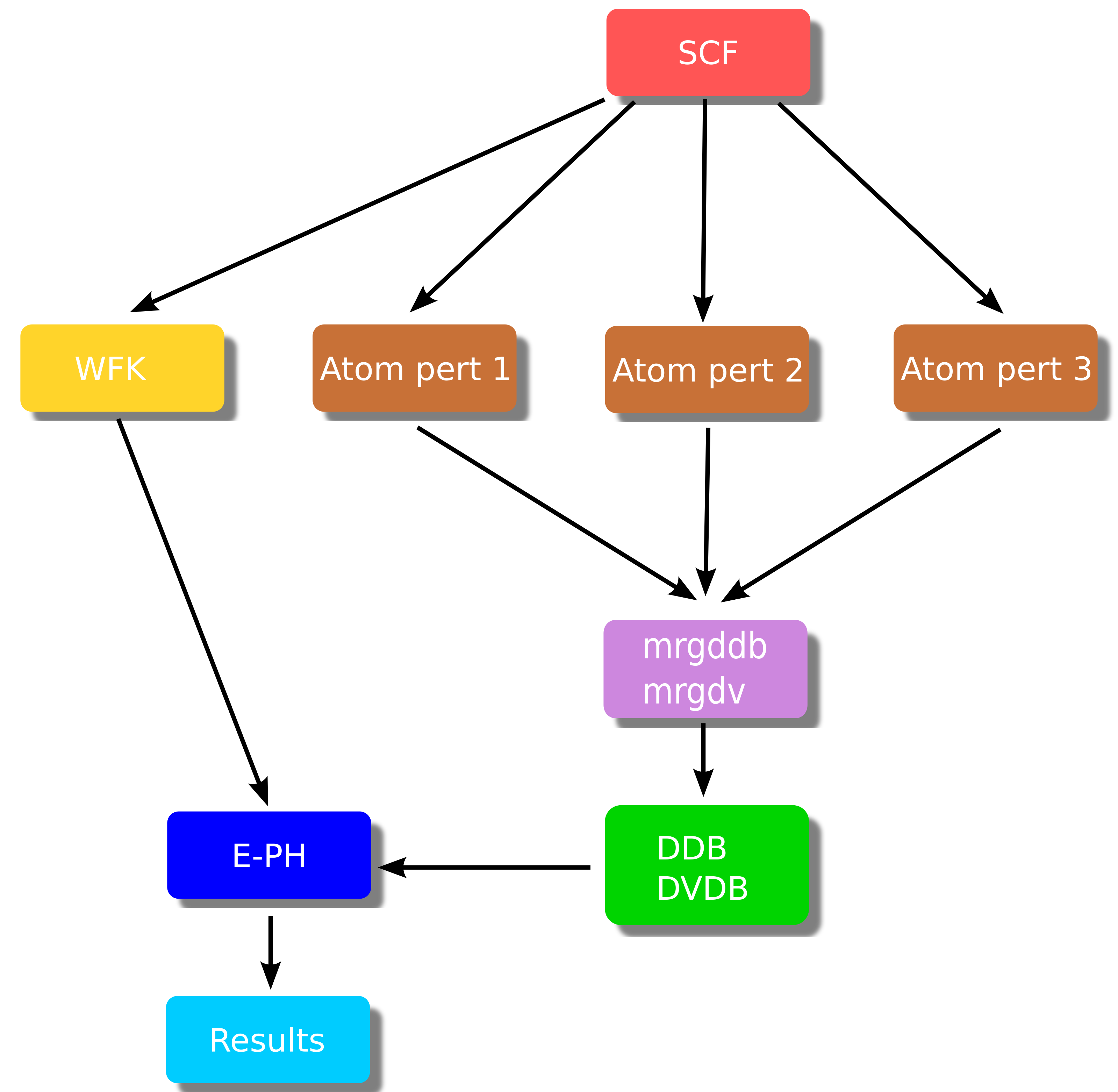
In order to perform a standard one-shot GW calculation one has to:

1. Run a converged ground state calculation to obtain the density.

2. Perform a non self-consistent run to compute the KS eigenvalues and the eigenfunctions including several empty states. Note that, unlike standard band structure calculations, here the KS states must be computed on a regular grid of k-points.

3. Use optdriver = 3 to compute the independent-particle susceptibility $\chi^0$ on a regular grid of q-points, for at least two frequencies (usually, $\omega=0$ and a purely imaginary frequency - of the order of the plasmon frequency, a dozen of eV).

The Green’s function is constructed from the KS wavefunctions and eigenvalues stored in the WFK file.

The following physical properties can be computed:

• Imaginary part of ph-e self-energy in metals (eph_task 1) that gives access to:

  • Phonon linewidths induced by e-ph coupling

• Real and imaginary parts of the e-ph self-energy (eph_task 4) that gives access to:

  • Zero-point renormalization of the band gap

At the time of writing, the following features are not yet supported in GWR:

• PAW calculations
• Spinors (nspinor = 2)

Tricks to accelerate the computation and reduce the memory requirements